Illustrative examples (INT12_08-15_COMPmay19_01-20)

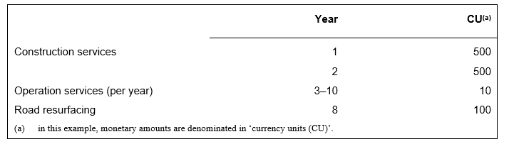
The terms of the arrangement require an operator to construct a road—completing construction within two years—and maintain and operate the road to a specified standard for eight years (ie years 3–10). The terms of the arrangement also require the operator to resurface the road at the end of year 8. At the end of year 10, the arrangement will end. Assume that the operator identifies three performance obligations for construction services, operation services and road resurfacing. The operator estimates that the costs it will incur to fulfil its obligations will be:

Table 1.1 Contract costs

The terms of the arrangement require the grantor to pay the operator 200 currency units (CU200) per year in years 3–10 for making the road available to the public.

For the purpose of this illustration, it is assumed that all cash flows take place at the end of the year.

The operator recognises revenue in accordance with AASB 15 Revenue from Contracts with Customers. Revenue—the amount of consideration to which the operator expects to be entitled from the grantor for the services provided—is recognised when (or as) the performance obligations are satisfied. Under the terms of the arrangement the operator is obliged to resurface the road at the end of year 8. In year 8 the operator will be reimbursed by the grantor for resurfacing the road.

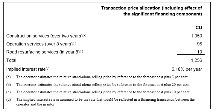
The total expected consideration (CU200 in each of years 3–10) is allocated to the performance obligations based on the relative stand-alone selling prices of the construction services, operation services and road resurfacing, taking into account the significant financing component, as follows:

Table 1.2 Transaction price allocated to each performance obligation

In year 1, for example, construction costs of CU500, construction revenue of CU525, and hence construction profit of CU25 are recognised in profit or loss.

During the first two years, the entity recognises a contract asset and accounts for the significant financing component in the arrangement in accordance with AASB 15. Once the construction is complete, the amounts due from the grantor are accounted for in accordance with AASB 9 Financial Instruments as receivables.

If the cash flows and fair values remain the same as those forecast, the effective interest rate is 6.18 per cent per year and the receivable recognised at the end of years 1–3 will be:

Table 1.3 Measurement of contract asset/receivable

For the purpose of this illustration, it is assumed that the operator finances the arrangement wholly with debt and retained profits. It pays interest at 6.7 per cent per year on outstanding debt. If the cash flows and fair values remain the same as those forecast, the operator’s cash flows, statement of comprehensive income and statement of financial position over the duration of the arrangement will be:

Table 1.4 Cash flows (currency units)

Table 1.5 Statement of comprehensive income (currency units)

Table 1.6 Statement of financial position (currency units)

This example deals with only one of many possible types of arrangements. Its purpose is to illustrate the accounting treatment for some features that are commonly found in practice. To make the illustration as clear as possible, it has been assumed that the arrangement period is only ten years and that the operator’s annual receipts are constant over that period. In practice, arrangement periods may be much longer and annual revenues may increase with time. In such circumstances, the changes in net profit from year to year could be greater.

The terms of a service arrangement require an operator to construct a road—completing construction within two years—and maintain and operate the road to a specified standard for eight years (ie years 3–10). The terms of the arrangement also require the operator to resurface the road when the original surface has deteriorated below a specified condition. The operator estimates that it will have to undertake the resurfacing at the end of year 8. At the end of year 10, the service arrangement will end. Assume that the operator identifies a single performance obligation for construction services. The operator estimates that the costs it will incur to fulfil its obligations will be:

Table 2.1 Contract costs

The terms of the arrangement allow the operator to collect tolls from drivers using the road. The operator forecasts that vehicle numbers will remain constant over the duration of the contract and that it will receive tolls of 200 currency units (CU200) in each of years 3–10.

For the purpose of this illustration, it is assumed that all cash flows take place at the end of the year.

The operator provides construction services to the grantor in exchange for an intangible asset, ie a right to collect tolls from road users in years 3–10. In accordance with AASB 15, the operator measures this non-cash consideration at fair value. In this case, the operator determines the fair value indirectly by reference to the stand-alone selling price of the construction services delivered.

During the construction phase of the arrangement the operator’s contract asset (representing its accumulating right to be paid for providing construction services) is presented as an intangible asset (licence to charge users of the infrastructure). The operator estimates the stand-alone selling price of the construction services to be equal to the forecast construction costs plus 5 per cent margin, which the operator concludes is consistent with the rate that a market participant would require as compensation for providing the construction services and for assuming the risk associated with the construction costs. It is also assumed that, in accordance with AASB 123 Borrowing Costs, the operator capitalises the borrowing costs, estimated at 6.7 per cent, during the construction phase of the arrangement:

Table 2.2 Initial measurement of intangible asset

In accordance with AASB 138, the intangible asset is amortised over the period in which it is expected to be available for use by the operator, ie years 3–10. The depreciable amount of the intangible asset (CU1,084) is allocated using a straight-line method. The annual amortisation charge is therefore CU1,084 divided by 8 years, ie CU135 per year.

The operator accounts for the construction services in accordance with AASB 15. It measures revenue at the fair value of the non-cash consideration received or receivable. Thus in each of years 1 and 2 it recognises in its profit or loss construction costs of CU500, construction revenue of CU525 and, hence, construction profit of CU25.

The road users pay for the public services at the same time as they receive them, ie when they use the road. The operator therefore recognises toll revenue when it collects the tolls.

The operator’s resurfacing obligation arises as a consequence of use of the road during the operating phase. It is recognised and measured in accordance with AASB 137 Provisions, Contingent Liabilities and Contingent Assets, ie at the best estimate of the expenditure required to settle the present obligation at the end of the reporting period.

For the purpose of this illustration, it is assumed that the terms of the operator’s contractual obligation are such that the best estimate of the expenditure required to settle the obligation at any date is proportional to the number of vehicles that have used the road by that date and increases by CU17 (discounted to a current value) each year. The operator discounts the provision to its present value in accordance with AASB 137. The charge recognised each period in profit or loss is:

Table 2.3 Resurfacing obligation (currency units)

For the purposes of this illustration, it is assumed that the operator finances the arrangement wholly with debt and retained profits. It pays interest at 6.7 per cent per year on outstanding debt. If the cash flows and fair values remain the same as those forecast, the operator’s cash flows, statement of comprehensive income and statement of financial position over the duration of the arrangement will be:

Table 2.4 Cash flows (currency units)

Table 2.5 Statement of comprehensive income (currency units)

Table 2.6 Statement of financial position (currency units)

This example deals with only one of many possible types of arrangements. Its purpose is to illustrate the accounting treatment for some features that are commonly found in practice. To make the illustration as clear as possible, it has been assumed that the arrangement period is only ten years and that the operator’s annual receipts are constant over that period. In practice, arrangement periods may be much longer and annual revenues may increase with time. In such circumstances, the changes in net profit from year to year could be greater.

The terms of a service arrangement require an operator to construct a road—completing construction within two years—and to operate the road and maintain it to a specified standard for eight years (ie years 3–10). The terms of the arrangement also require the operator to resurface the road when the original surface has deteriorated below a specified condition. The operator estimates that it will have to undertake the resurfacing at the end of year 8. At the end of year 10, the arrangement will end. Assume that the operator identifies a single performance obligation for construction services. The operator estimates that the costs it will incur to fulfil its obligations will be:

Table 3.1 Contract costs

The operator estimates the consideration in respect of construction services to be CU1,050 by reference to the stand-alone selling price of those services (which it estimates at forecast cost plus 5 per cent).

The terms of the arrangement allow the operator to collect tolls from drivers using the road. In addition, the grantor guarantees the operator a minimum amount of CU700 and interest at a specified rate of 6.18 per cent to reflect the timing of cash receipts. The operator forecasts that vehicle numbers will remain constant over the duration of the contract and that it will receive tolls of CU200 in each of years 3–10.

For the purpose of this illustration, it is assumed that all cash flows take place at the end of the year.

The contractual right to receive cash from the grantor for the services and the right to charge users for the public services should be regarded as two separate assets under Australian Accounting Standards. Therefore in this arrangement it is necessary to divide the operator’s contract asset during the construction phase into two components—a financial asset component based on the guaranteed amount and an intangible asset for the remainder. When the construction services are completed, the two components of the contract asset would be classified and measured as a financial asset and an intangible asset accordingly.

Table 3.2 Dividing the operator’s consideration

During the first two years, the entity recognises a contract asset and accounts for the significant financing component in the arrangement in accordance with AASB 15. Once the construction is complete, the amount due from, or at the direction of, the grantor in exchange for the construction services is accounted for in accordance with AASB 9 as a receivable.

On this basis the receivable recognised at the end of years 2 and 3 will be:

Table 3.3 Measurement of contract asset/receivable

In accordance with AASB 138 Intangible Assets, the operator recognises the intangible asset at cost, ie the fair value of the consideration received or receivable.

During the construction phase of the arrangement the portion of the operator’s contract asset that represents its accumulating right to be paid amounts in excess of the guaranteed amount for providing construction services is presented as a right to receive a licence to charge users of the infrastructure. The operator estimates the stand-alone selling price of the construction services as equal to the forecast construction costs plus 5 per cent, which the operator concludes is consistent with the rate that a market participant would require as compensation for providing the construction services and for assuming the risk associated with the construction costs. It is also assumed that, in accordance with AASB 123 Borrowing Costs, the operator capitalises the borrowing costs, estimated at 6.7 per cent, during the construction phase:

Table 3.4 Initial measurement of intangible asset

In accordance with AASB 138, the intangible asset is amortised over the period in which it is expected to be available for use by the operator, ie years 3–10. The depreciable amount of the intangible asset (CU361 including borrowing costs) is allocated using a straight-line method. The annual amortisation charge is therefore CU361 divided by 8 years, ie CU45 per year.

The operator provides construction services to the grantor in exchange for a financial asset and an intangible asset. Under both the financial asset model and intangible asset model, the operator accounts for the construction services in accordance with AASB 15. Thus in each of years 1 and 2 it recognises in profit or loss construction costs of CU500 and construction revenue of CU525.

The road users pay for the public services at the same time as they receive them, ie when they use the road. Under the terms of this arrangement the cash flows are allocated to the financial asset and intangible asset in proportion, so the operator allocates the receipts from tolls between repayment of the financial asset and revenue earned from the intangible asset:

Table 3.5 Allocation of toll receipts

The operator’s resurfacing obligation arises as a consequence of use of the road during the operation phase. It is recognised and measured in accordance with AASB 137 Provisions, Contingent Liabilities and Contingent Assets, ie at the best estimate of the expenditure required to settle the present obligation at the end of the reporting period.

For the purpose of this illustration, it is assumed that the terms of the operator’s contractual obligation are such that the best estimate of the expenditure required to settle the obligation at any date is proportional to the number of vehicles that have used the road by that date and increases by CU17 each year. The operator discounts the provision to its present value in accordance with AASB 137. The charge recognised each period in profit or loss is:

Table 3.6 Resurfacing obligation (currency units)

For the purposes of this illustration, it is assumed that the operator finances the arrangement wholly with debt and retained profits. It pays interest at 6.7 per cent per year on outstanding debt. If the cash flows and fair values remain the same as those forecast, the operator’s cash flows, statement of comprehensive income and statement of financial position over the duration of the arrangement will be:

Table 3.7 Cash flows (currency units)

Table 3.8 Statement of comprehensive income (currency units)

Table 3.9 Statement of financial position (currency units)

This example deals with only one of many possible types of arrangements. Its purpose is to illustrate the accounting treatment for some features that are commonly found in practice. To make the illustration as clear as possible, it has been assumed that the arrangement period is only ten years and that the operator’s annual receipts are constant over that period. In practice, arrangement periods may be much longer and annual revenues may increase with time. In such circumstances, the changes in net profit from year to year could be greater.